Content for TS 22.104 Word version: 19.2.0
0f…
4…
5…
5.3…
6…
A…
A.2.2…
A.2.2.4…
A.2.3…
A.4…
A.4.4…
A.4.4.3…
A.4.5…
A.4.8…
A.5…
A.6…
B…
C…
C.3
C.4…
C.5
D…
E…
A.4.5 Smart grid millisecond-level precise load control
A.4.6 Distributed energy storage
A.4.7 Advanced metering
...
...
A.4.5 Smart grid millisecond-level precise load control p. 63
Precise Load Control is the basic application for smart grid. When serious HVDC (high-voltage direct current) transmission fault happens, Millisecond-Level Precise Load Control is used to quickly remove interruptible less-important load, such as electric vehicle charging piles and non-continuous production power supplies in factories.
| Use case # | Characteristic parameter | Influence quantity | ||||||||
|---|---|---|---|---|---|---|---|---|---|---|
| Communication service availability: target value in % | Communication service reliability: mean time between failures | End-to-end latency: maximum | Service bitrate: user experienced data rate | Message size [byte] | Transfer interval: target value | Survival time | UE speed | # of UEs | Service area | |
| 1 | 99.999 9 | – | < 50 ms | 0.59 kbit/s 28 kbit/s | < 100 | n/a (note) | – | stationary | 10 km² to 100 km² | TBD |
|
NOTE:
event-triggered
|
||||||||||
Use case one
A non-periodic deterministic communication service between control primary station and load control terminals for removing interruptible less-important load quickly.
A.4.6 Distributed energy storage |R18| p. 65
Distributed power generation includes various power sources such as solar, wind, fuel cells, and gas. Distributed power generation typically comes with a low power density and entails thus typicall a decentralised deployment. Decentralisation causes technical problems and challenges Smart Grid operators. When distributed power generation is connected to the elctrical grid, the energy flow becomes more complicated as the user often is both an electricity consumer and producer (a so-called "prosumer"). Therefore, the current in the electricity grid can change direction at different locations of the grid and at different times of the day.
The information exchange in a distributed energy grid does not only include power-generation-related data, but also control commands for the distributed energy storage equipment. An example for such a command is "change the load characteristics to realise a flexible electricity grid" etc.
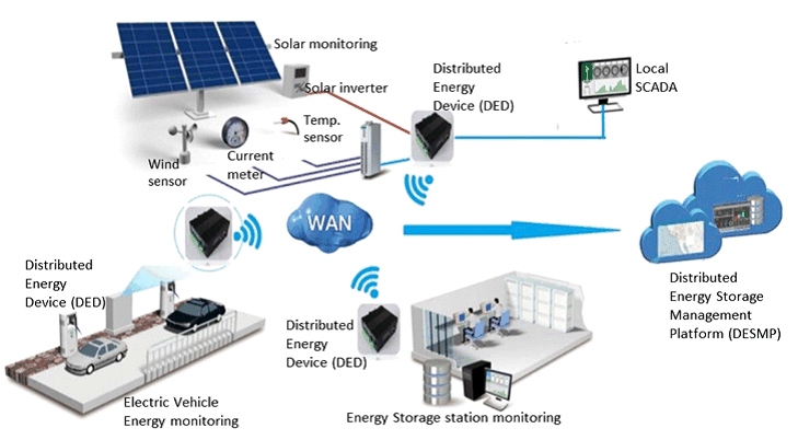
Figure A.4.6-1 shows an example of distributed-energy storage grid. The distributed-energy storage grid needs to exchange information among the distributed-energy storage management platform (DESMP) and distributed-energy devices (DEDs).
The DED is a plug-and-play device and periodically collects its energy information, such as battery energy, charge and discharge status, energy alarm information, etc. The DED then transfers this information via 5G UE to the DESMP. The DESMP regularly manages the DEDs, e.g., the DESMP monitors the DEDs working status, controls the DEDs working modes, or configures the DEDs energy parameters etc. The associated KPIs are provided in Table A.4.6-1.
| Use case # | Characteristic parameter | Influence quantity | ||||||||
|---|---|---|---|---|---|---|---|---|---|---|
| Communication service availability: target value | Communication service reliability: mean time between failures | End-to-end latency: maximum | Service bitrate: user experienced data rate | Message size [byte] | Transfer interval: target value | Survival time | UE speed | # of UEs | Service area | |
| 1 | > 99.9 % | – | DL: < 10 ms UL: < 10 ms | UL: > 16 Mbit/s (urban); 640 Mbit/s (rural) DL: > 100 kbit/s (note 1) | UL: 800 kbyte | UL: 10 ms | – | stationary | > 10/km² (urban); > 100/km² (rural) (note 2) | several km² |
| 2 | > 99.9 % | – | DL: < 10 ms UL: < 1 s | UL: > 128 kbit/s (urban); 10.4 Mbit/s (rural); DL: > 100 kbit/s (note 1) | UL: 1.3 Mbyte DL: > 100 kbyte | UL: 1000 ms | – | stationary | > 10/km² (urban); > 100/km² (rural) (note 2) | several km² |
| 3 | > 99.9 % | – | DL: < 10 ms UL:< 1 s (rural) | DL: > 100 kbit/s UL: > 5 Gbit/s (note 3) | stationary | > 100/km² | several km² | |||
|
NOTE 1:
Service bit rate for one energy storage station.
NOTE 2:
Activity storage nodes/km². This value is used for deducing the data volume in an area that features multiple energy storage stations. The data volume can be calculated with the following formula (current service bit rate per storage station) x (activity storage nodes/km²) + (video service bit rate per storage station) x (activity storage nodes/km²).
NOTE 3:
The downlink user experienced data rate is calculated as follows: 12.5 Mbytes/s x 50(containers) x 8 = 5 Gbit/s
|
||||||||||
Use case#1:
Distributed energy storage - periodic communication for monitoring
Use case#2:
Distributed energy storage - periodic communication for data collection
Use case#3:
Distributed energy storage - aperiodic video communication
A.4.7 Advanced metering |R18| p. 67
Instead of recording and sending metering data from a wired electricity meter unit, electricity metering collecting can be executed by a UE-integrated smart meter unit. Smart meter units can send real-time metering data to a server in the utility through mobile networks. In this way, the power enterprise - based on the analysis of the user's power consumption behavior - gives the user power consumption suggestions, which fosters the user's power consumption and energy saving habits.
The electric smart meters monitor relevant user energy status and deliver the status data to a measurement data management system (MDMS). The MDMS sends control commands according to its policy and the status of the data collected from the smart meters. The MDMS commands include tripping, closing permission, alarm, alarm release, power protection, and power protection release. Accurate-fee control is one of the basic services of advanced metering. When the electric power user doesn't pay her electric fee on time, the MDMS can cut off the power supply. And when there is a need for temporary power supply for this user, the MDMS can recover the power supply. This operation requires real-time interaction between the electric smart meter and the MDMS. Due to massive number of electricity meters, it is estimated that in the near future, the amount of this kind of interaction will increase 5 to 10 times. The associated KPIs are provided in Table A.4.7-1.
| Use case # | Characteristic parameter | Influence quantity | ||||||||
|---|---|---|---|---|---|---|---|---|---|---|
| Communication service availability: target value | Communication service reliability: mean time between failures | End-to-end latency: maximum | Service bitrate: user experienced data rate | Message size [byte] | Transfer interval: target value | Survival time | UE speed | # of UEs | Service area | |
| 1 | > 99.99 | – | Accuracy fee control: < 100 (note 1); General information data collection: < 3000 | UL: < 2 M DL: < 1 M | – | – | – | stationary | < 10 000/km2 (note2) | – |
|
NOTE 1:
One-way delay from 5G IoT device to backend system. The distance between the two is below 40 km (city range).
NOTE 2:
It is the typical connection density in today city environment. With the evolution from centralised meters to socket meters in the home, the connection density is expected to increase 5 to 10 times.
|
||||||||||
Use case#1:
Advanced metering
![]()
![]()
![]()