Content for TR 26.928 Word version: 17.0.0
0…
4…
4.1.2…
4.2…
4.3…
4.4…
4.5…
4.6…
4.6.7
4.7…
4.9…
5…
6…
7…
8
A…
A.4…
A.7…
A.10…
A.13
A.14
A.15
A.16…
A.19…
A.22…
4.6 3D and XR Visual Formats
4.6.1 Introduction
4.6.2 Omnidirectional Visual Formats
4.6.2.1 Introduction
4.6.2.2 Definition
4.6.2.3 Production and Capturing Systems
4.6.2.4 Rendering
4.6.2.5 Compression, Storage and Data Formats
4.6.2.6 Quality and Bitrate considerations
4.6.2.7 Applications
4.6.3 3D Meshes
4.6.3.1 Introduction
4.6.3.2 Definition
4.6.3.3 Production and Capturing Systems
4.6.3.4 Rendering
4.6.3.5 Storage and Data Formats
4.6.3.6 Texture Formats
4.6.3.8 Bitrate and Quality Considerations
4.6.3.7 Applications
4.6.4 Point Clouds
4.6.5 Light Fields
4.6.6 Scene Description
...
...
4.6 3D and XR Visual Formats p. 34
4.6.1 Introduction p. 34
This clause introduces 3D and XR visual formats. Both, static images as well as video formats are introduced. In all cases it is assumed that the visual signal is provided as a sequence of pictures with a specific frame rate in frames per second. The chosen frame rate may be a matter of the production of the video, or it may be based on requirements due to interactions with the content, for example in case of conversational applications or when using split rendering.
4.6.2 Omnidirectional Visual Formats p. 34
4.6.2.1 Introduction p. 34
Omnidirectional formats have been introduced in clause 4.1 of TS 26.118, as well as in clause 4.2.5 of TR 26.918.
4.6.2.2 Definition p. 34
Omnidirectional visual signals are represented in a spherical coordinate space in angular coordinates (ϕ,θ). The viewing is from the origin of the sphere, looking outward. Even though a spherical coordinate is generally represented by using radius, elevation, and azimuth, it assumes that a unit sphere is used for capturing and rendering. Thus, a location of a point on the unit sphere is identified by using the sphere coordinates azimuth (ϕ) and elevation (θ).
For video, such a centre point may exist for each eye, referred to as stereo signal, and the video consists of three colour components, typically expressed by the luminance (Y) and two chrominance components (U and V).
According to clause 4.1.3 of TS 26.118, mapping of a spherical picture to a 2D texture signal is illustrated in Figure 4.6.2-1. The most commonly used mapping from spherical to 2D is the equirectangular projection (ERP) mapping. The mapping is bijective, i.e. it may be expressed in both directions.
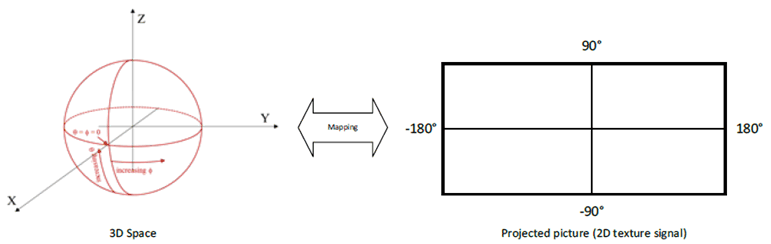
Assume a 2D texture with pictureWidth and pictureHeight, being the width and height, respectively, of a monoscopic projected luma picture, in luma samples and the center point of a sample location (i,j) along the horizontal and vertical axes, respectively, then for the equirectangular projection the sphere coordinates (ϕ,θ) for the luma sample location, in degrees, are given by the following equations:
ϕ = ( 0.5 − i ÷ pictureWidth ) * 360
θ = ( 0.5 − j ÷ pictureHeight ) * 180
Whereas ERP is commonly used for production formats, other mappings may be applied, especially for distribution. For more details on projection formats, refer to clause 4.2.5.4 of TR 26.918.
4.6.2.3 Production and Capturing Systems p. 35
For production, capturing and stitching of spherical content, refer to clauses 4.2.5.2 and 4.2.5.3 of TR 26.918.
4.6.2.4 Rendering p. 35
Rendering of spherical content depends on the field of view (FoV) of a rendering device. The pose together with the field of view of the device enables the system to generate the user viewport, i.e., the presented part of the content at a specific point in time. According to TS 26.118, the renderer uses the projected texture signals and rendering metadata (projection information) and provides a viewport presentation taking into account the viewport and possible other information. With the pose, a user viewport is determined by identifying the horizontal and vertical fields of view of the screen of a head-mounted display or any other display device to render the appropriate part of decoded video or audio signals. For video, textures from decoded signals are projected to the sphere with rendering metadata received from the file decoder. During the texture-to-sphere mapping, a sample of the decoded signal is remapped to a position on the sphere.
Related to the generic rendering approaches in clause 4.2.2, the following steps are part of the rendering spherical media:
- Generating a 3D Mesh (set of vertexes linked into triangles) based on the projection metadata. The sphere is mapped to a mesh and the transformation of the mesh is dynamically updated based on the updated projection metadata.
- Mapping each vertex to a position on a 2D texture. This is again done using the available projection metadata.
- Rotating the camera to match the user's head orientation. This is based on the available pose information.
- Computing the viewport by using computer graphic algorithms as discussed in details in clause 4.2.2
4.6.2.5 Compression, Storage and Data Formats p. 35
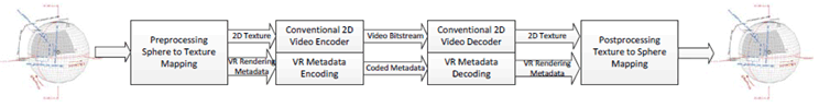
According to clause 4.1.3 of TS 26.118, commonly used video encoders cannot directly encode spherical videos, but only 2D textures. However, there is a significant benefit to reuse conventional 2D video encoders. Based on this, Figure 4.6.2-2 provides the basic video signal representation in the context of omnidirectional video in the context of the present document. By pre-processing, the spherical video is mapped to a 2D texture. The 2D texture is encoded with a regular 2D video encoder and the VR rendering metadata (i.e. the data describing the mapping from the spherical coordinate to the 2D texture) is encoded and provided along with the video bitstream, such that at the receiving end the inverse process can be applied to reconstruct the spherical video.
Compression, storage and data formats are defined for example in TS 26.118 as well as in ISO/IEC 23090-2 [37]. This includes viewport-independent and viewport-dependent compression formats. A principle overview of different approaches is documented in clause 4.2.5.6 of TR 26.918.
4.6.2.6 Quality and Bitrate considerations p. 36
According to clause 4.2.1, 1k by 1k per eye is a minimum for the signal in the viewport, and for stereoscopic rendering this results in basically a signal for 2k by 1k, typically at a frame rate of 50 or 60fps.With current codecs according to clause 4.5.1, the pure viewport data can be represented with around 4-10 Mbit/s. However, a viewport typically only covers around 100 degree horizontal and 60 degree vertical. Hence, to present a full omnidirectional presentation, about 20 times more data may be necessary, leading to 80 - 200 Mbit/s. Viewport-dependent coding and delivery, in particular tiling, can support to reduce the required bitrates.
4.6.2.7 Applications p. 36
For use cases and applications, see clause 5 of TR 26.918.
4.6.3 3D Meshes p. 36
4.6.3.1 Introduction p. 36
A polygon mesh is a collection of vertices, edges and faces that defines the shape of a polyhedral object in 3D computer graphics and solid modeling. The faces usually consist of triangles (triangle mesh), quadrilaterals (quads), or other simple convex polygons (n-gons), since this simplifies rendering, but may also be more generally composed of concave polygons, or even polygons with holes.
4.6.3.2 Definition p. 36
Objects created with polygon meshes are represented by different types of elements. These include vertices, edges, faces, polygons and surfaces as shown in Figure 4.6.3-1. In many applications, only vertices, edges and either faces or polygons are stored.
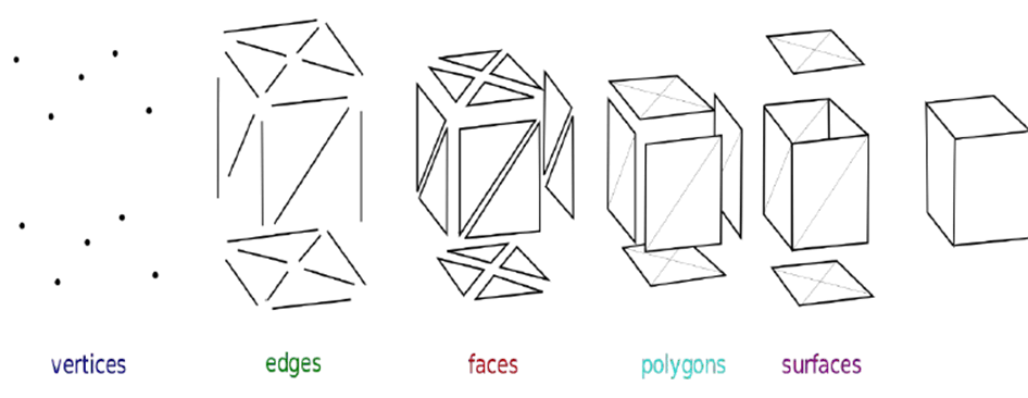
Figure 4.6.3-1: Elements necessary for mesh representations ©Wikipedia
(⇒ copy of original 3GPP image)
(⇒ copy of original 3GPP image)
(Mesh_overview.jpg: The original uploader was Rchoetzlein at English Wikipedia.derivative work: Lobsterbake [CC BY-SA 3.0 (https://creativecommons.org/licenses/by-sa/3.0 )])
Polygon meshes are defined by the following elements:
- Vertex: A position in 3D space defined as (x,y,z) along with other information such as colour (r,g,b), normal vector and texture coordinates.
- Edge: A connection between two vertices.
- Face: A closed set of edges, in which a triangle face has three edges, and a quad face has four edges. A polygon is a coplanar set of faces. In systems that support multi-sided faces, polygons and faces are equivalent. Mathematically a polygonal mesh may be considered as an unstructured grid, or undirected graph, with additional properties of geometry, shape and topology.
- Surfaces: or smoothing groups, are useful, but not required to group smooth regions.
- Groups: Some mesh formats contain groups, which define separate elements of the mesh, and are useful for determining separate sub-objects for skeletal animation or separate actors for non-skeletal animation.
- Materials: defined to allow different portions of the mesh to use different shaders when rendered.
- UV coordinates: Most mesh formats also support some form of UV coordinates which are a separate 2D representation of the mesh "unfolded" to show what portion of a 2-dimensional texture map to apply to different polygons of the mesh. It is also possible for meshes to contain other such vertex attribute information such as colour, tangent vectors, weight maps to control animation, etc (sometimes also called channels).
4.6.3.3 Production and Capturing Systems p. 37
Meshes are commonly produced by many different graphics engines, computer games, and so on. For more details, see also clause 4.6.7.
4.6.3.4 Rendering p. 37
Meshes can be rendered directly on GPUs that are highly optimized for mesh-based rendering.
4.6.3.5 Storage and Data Formats p. 37
4.6.3.5.1 Introduction p. 37
Polygon meshes may be represented in a variety of ways, using different methods to store the vertex, edge and face data such as face-vertex, winged, half or quad-edge meshes, corner-table or vertex-vertex meshes. Different formats also store other per vertex and materials related data in different ways. Each of the representations have particular advantages and drawbacks. The choice of the data structure is governed by the application, the required performance, the size of the data, and the operations to be performed. For example, it is easier to deal with triangles than general polygons. For certain operations it is necessary to have a fast access to topological information such as edges or neighboring faces; this requires more complex structures such as the winged-edge representation. For hardware rendering, compact, simple structures are needed and are as such commonly incorporated into low-level rendering APIs such as DirectX and OpenGL.
Many different formats for storage and data formats exist for storing polygon mesh data, as an example PLY-format is introduced below, because it provides 3D data in a human readable format. In practice PLY-format is rarely used in real-time rendering. Typically the data format is configured to the need of the 3D engine and as such the landscape is littered with proprietary 3D formats. 3D formats may be roughly divided in two categories, run time friendly formats such as glTF and formats which enable transferring 3D assets between systems like PLY.
4.6.3.5.2 PoLYgon (PLY) File Format p. 37
The PoLYgon (PLY) format (see http://paulbourke.net/dataformats/ply/ ) is used to describe a 3D object as a list of vertices, faces and other elements, along with associated attributes. A single PLY file describes exactly one 3D object. The 3D object may be generated synthetically or captured from a real scene. Attributes of the 3D object elements that might be stored with the object include: colour, surface normals, texture coordinates, transparency, etc. The format permits one object to have different properties for the front and back of a polygon.
The PLY does not intend to act as a Scene Graph, so it does not include transformation matrices, multiple 3D objects, modeling hierarchies, or object sub-parts. A typical PLY object definition is a list of (x,y,z,r,g,b) triples for vertices and their colour attributes (r,g,b), so they represent a point cloud. It may also include a list of faces that are described by indices into the list of the vertices. Vertices and faces are primary elements of the 3D object representation.
PLY allows applications to create new attributes that are attached to the elements of an object. New attributes are appended to the list of attributes of an element, in a way to maintain backwards compatibility. Attributes that are not understood by a parser are simply skipped.
Furthermore, PLY allows for extensions to create new element types and their associated attributes. Examples of such elements could be materials (ambient, diffuse and specular colours and coefficients). New elements can also be discarded by programs that do not understand them.
A PLY file is structured as follows:
  Header
  Vertex List
  Face List
  (lists of other elements)
The header is a human-readable textual description of the PLY file. It contains a description of each element type, including the element's name (e.g. "vertex"), how many of such elements are in the object, and a list of the various attributes associated with the element. The header also indicates whether the file is in binary or ASCII format. A list of elements for each element type follows the header in the order described in the header. The following is an example PLY in binary format with 19928 vertices and 39421 faces: This example demonstrates the different components of a PLY file header. Each part of the header is a carriage-return terminated ASCII string that begins with a keyword. In case of binary representation, the file will be a mix of an ASCII header and binary representation of the elements, in little or big endian, depending on the architecture on which the PLY file has been generated. The PLY file must start with the characters "ply". The vertex attributes listed in this example are the (x,y,z) floating point coordinates, the (nx,ny,nz) representation of the normal vectors, a 32 bit flag mask, (r,g,b) 8-bit representations of the colour of each vertex, an 8-bit representation of the transparency alpha channel. Faces are represented as a list of vertex indices with a flags attribute associated with each face.
4.6.3.6 Texture Formats p. 38
Different GPUs may support different texture formats, both raw and compressed. Raw formats include different representations of the RGB colour space, e.g. 8/16/32 bit representations of each colour component, with or without alpha channel, float or integer, regular or normalized, etc.
Typical GPU texture compression formats include BC1, PVRTC, ETC2/EAC, and ASTC. Other image compression formats such as JPEG and PNG need to be decompressed and passed to the GPU in a format that it supports.
Recently, the Basis Universal GPU texture format has been defined. This format also supports video texture compression. As decoding happens on the GPU, the application will benefit from reduced CPU load and CPU to GPU memory copy delay.
4.6.3.8 Bitrate and Quality Considerations p. 38
Bitrates and quality considerations for meshes are FFS.
4.6.3.7 Applications p. 39
Meshes are used in many applications.
4.6.4 Point Clouds p. 39
A point cloud is a collection of data points defined by a given coordinates system. In a 3D coordinates system, for example, a point cloud may define the shape of some real or created physical system. Point clouds are used to create 3D meshes and other models used in 3D modeling for various fields including medical imaging, architecture, 3D printing, manufacturing, 3D gaming and various XR applications.
Point clouds are often aligned with 3D models or with other point clouds, a process known as point set registration. In computer vision and pattern recognition, point set registration, also known as point matching, is the process of finding a spatial transformation that aligns two-point sets. The purpose of finding such a transformation includes merging multiple data sets into a globally consistent model, and mapping a new measurement to a known data set to identify features or to estimate its pose. Point set registration is used in augmented reality.
An overview on point cloud definitions, formats, production and capturing systems, rendering, bitrate/quality considerations and applications is for example provided in [38]. According to this document, media-related use cases may usually contain between 100,000 and 10,000,000 point locations and colour attributes with 8-10 bits per colour component, along with as some sort of temporal information, similar to frames in a video sequence. For navigation purposes, it is possible to generate a 3D map by combining depth measurements from a high-density laser scanner, e.g. LIDAR, camera captured images and localization data measured with GPS and an inertial measurement unit (IMU). Such maps can further be combined with road markings such as lane information and road signs to create maps to enable autonomous navigation of vehicles around a city. This use case requires the capture of millions to billions of 3D points with up to 1 cm precision, together with additional attributes, namely colour with 8-12 bits per colour component, surface normals and reflectance properties attributes. According to the paper, depending on the sequence, compression factors between 1:100 to 1:500 are feasible for media-related applications. According to the same paper, bitrates for single objects with such compression methods are in the range of 8 to 20 Mbit/s.
For production of point clouds, see also clause 4.6.7.
4.6.5 Light Fields p. 39
An overview on light-field technology is for example provided in https://mpeg.chiariglione.org/sites/default/files/events/7.%20MPEG127-WS_MehrdadTeratani.pdf .
4.6.6 Scene Description p. 39
Scene Descriptions are often called scene graphs due to their representation as graphs. A scene graph is a directed acyclic graph, usually just a plain tree-structure, that represents an object-based hierarchy of the geometry of a scene. The leaf nodes of the graph represent geometric primitives such as polygons. Each node in the graph holds pointers to its children. The child nodes can among others be a group of other nodes, a geometry element, a transformation matrix, etc.
Spatial transformations are represented as nodes of the graph and represented by a transformation matrix. Other Scene Graph nodes include 3D objects or parts thereof, light sources, particle systems, viewing cameras, …
This structure of scene graphs has the advantage of reduced processing complexity, e.g. while traversing the graph for rendering. An example operation that is simplified by the graph representation is the culling operation, where branches of the graph are dropped from processing, if deemed that the parent node's space is not visible or relevant (level of detail culling) to the rendering of the current view frustum.
Scene descriptions permit generation of many different 3D scenes for XR applications. As an example, glTF from Khronos [39] is a widely adopted scene description specification and is now adopted by MPEG as the baseline for their extensions to integrate real-time media into scenes.
![]()
![]()
![]()